Example 0: The Simplest Neuroptimiser
This example demonstrates how to use the Neuroptimiser library to solve a dummy optimisation problem.
1. Setup
Import minimal necessary libraries.
import matplotlib.pyplot as plt
import numpy as np

from neuroptimiser import NeurOptimiser
2. Quick problem and optimiser setup
We define a simple optimisation problem with a fitness function and bounds.
problem_function    = lambda x: np.linalg.norm(x)
problem_bounds      = np.array([[-5.0, 5.0], [-5.0, 5.0]])
Then, we instantiate the Neuroptimiser with the default configurations.
optimiser = NeurOptimiser()
#optimiser = NeurOptimiser(core_params={"hs_operator": "directional", "hs_variant": "pbest"})
# selector_params={"sel_mode": "greedy"}
# Show the overall configuration parameters of the optimiser
print("DEFAULT CONFIG PARAMS:\n", optimiser.config_params, "\n")
print("DEFAULT CORE PARAMS:\n", optimiser.core_params)
print("\nDEFAULT HIGH-LEVEL SELECTOR PARAMS:\n", optimiser.selector_params, "\n")
DEFAULT CONFIG PARAMS:
 {'num_dimensions': 2, 'seed': 69, 'num_neighbours': 1, 'neuron_topology': '2dr', 'unit_topology': '2dr', 'search_space': array([[-1,  1],
       [-1,  1]]), 'spiking_core': 'TwoDimSpikingCore', 'function': None, 'num_iterations': 300, 'core_params': {}, 'num_agents': 10}

DEFAULT CORE PARAMS:
 [{'spk_q_ord': 2, 'thr_max': 1.0, 'is_bounded': False, 'sel_mode': 'greedy', 'seed': None, 'max_steps': 100, 'spk_alpha': 0.25, 'alpha': 1.0, 'hs_params': {}, 'approx': 'rk4', 'thr_k': 0.05, 'dt': 0.01, 'thr_min': 1e-06, 'thr_alpha': 1.0, 'spk_cond': 'l1', 'name': 'linear', 'thr_mode': 'diff_pg', 'hs_operator': 'differential', 'noise_std': 0.1, 'coeffs': 'random', 'ref_mode': 'pgn', 'spk_weights': [0.5, 0.5], 'hs_variant': 'rand'}, {'spk_q_ord': 2, 'thr_max': 1.0, 'is_bounded': False, 'sel_mode': 'greedy', 'seed': None, 'max_steps': 100, 'spk_alpha': 0.25, 'alpha': 1.0, 'hs_params': {}, 'approx': 'rk4', 'thr_k': 0.05, 'dt': 0.01, 'thr_min': 1e-06, 'thr_alpha': 1.0, 'spk_cond': 'l1', 'name': 'linear', 'thr_mode': 'diff_pg', 'hs_operator': 'differential', 'noise_std': 0.1, 'coeffs': 'random', 'ref_mode': 'pgn', 'spk_weights': [0.5, 0.5], 'hs_variant': 'rand'}, {'spk_q_ord': 2, 'thr_max': 1.0, 'is_bounded': False, 'sel_mode': 'greedy', 'seed': None, 'max_steps': 100, 'spk_alpha': 0.25, 'alpha': 1.0, 'hs_params': {}, 'approx': 'rk4', 'thr_k': 0.05, 'dt': 0.01, 'thr_min': 1e-06, 'thr_alpha': 1.0, 'spk_cond': 'l1', 'name': 'linear', 'thr_mode': 'diff_pg', 'hs_operator': 'differential', 'noise_std': 0.1, 'coeffs': 'random', 'ref_mode': 'pgn', 'spk_weights': [0.5, 0.5], 'hs_variant': 'rand'}, {'spk_q_ord': 2, 'thr_max': 1.0, 'is_bounded': False, 'sel_mode': 'greedy', 'seed': None, 'max_steps': 100, 'spk_alpha': 0.25, 'alpha': 1.0, 'hs_params': {}, 'approx': 'rk4', 'thr_k': 0.05, 'dt': 0.01, 'thr_min': 1e-06, 'thr_alpha': 1.0, 'spk_cond': 'l1', 'name': 'linear', 'thr_mode': 'diff_pg', 'hs_operator': 'differential', 'noise_std': 0.1, 'coeffs': 'random', 'ref_mode': 'pgn', 'spk_weights': [0.5, 0.5], 'hs_variant': 'rand'}, {'spk_q_ord': 2, 'thr_max': 1.0, 'is_bounded': False, 'sel_mode': 'greedy', 'seed': None, 'max_steps': 100, 'spk_alpha': 0.25, 'alpha': 1.0, 'hs_params': {}, 'approx': 'rk4', 'thr_k': 0.05, 'dt': 0.01, 'thr_min': 1e-06, 'thr_alpha': 1.0, 'spk_cond': 'l1', 'name': 'linear', 'thr_mode': 'diff_pg', 'hs_operator': 'differential', 'noise_std': 0.1, 'coeffs': 'random', 'ref_mode': 'pgn', 'spk_weights': [0.5, 0.5], 'hs_variant': 'rand'}, {'spk_q_ord': 2, 'thr_max': 1.0, 'is_bounded': False, 'sel_mode': 'greedy', 'seed': None, 'max_steps': 100, 'spk_alpha': 0.25, 'alpha': 1.0, 'hs_params': {}, 'approx': 'rk4', 'thr_k': 0.05, 'dt': 0.01, 'thr_min': 1e-06, 'thr_alpha': 1.0, 'spk_cond': 'l1', 'name': 'linear', 'thr_mode': 'diff_pg', 'hs_operator': 'differential', 'noise_std': 0.1, 'coeffs': 'random', 'ref_mode': 'pgn', 'spk_weights': [0.5, 0.5], 'hs_variant': 'rand'}, {'spk_q_ord': 2, 'thr_max': 1.0, 'is_bounded': False, 'sel_mode': 'greedy', 'seed': None, 'max_steps': 100, 'spk_alpha': 0.25, 'alpha': 1.0, 'hs_params': {}, 'approx': 'rk4', 'thr_k': 0.05, 'dt': 0.01, 'thr_min': 1e-06, 'thr_alpha': 1.0, 'spk_cond': 'l1', 'name': 'linear', 'thr_mode': 'diff_pg', 'hs_operator': 'differential', 'noise_std': 0.1, 'coeffs': 'random', 'ref_mode': 'pgn', 'spk_weights': [0.5, 0.5], 'hs_variant': 'rand'}, {'spk_q_ord': 2, 'thr_max': 1.0, 'is_bounded': False, 'sel_mode': 'greedy', 'seed': None, 'max_steps': 100, 'spk_alpha': 0.25, 'alpha': 1.0, 'hs_params': {}, 'approx': 'rk4', 'thr_k': 0.05, 'dt': 0.01, 'thr_min': 1e-06, 'thr_alpha': 1.0, 'spk_cond': 'l1', 'name': 'linear', 'thr_mode': 'diff_pg', 'hs_operator': 'differential', 'noise_std': 0.1, 'coeffs': 'random', 'ref_mode': 'pgn', 'spk_weights': [0.5, 0.5], 'hs_variant': 'rand'}, {'spk_q_ord': 2, 'thr_max': 1.0, 'is_bounded': False, 'sel_mode': 'greedy', 'seed': None, 'max_steps': 100, 'spk_alpha': 0.25, 'alpha': 1.0, 'hs_params': {}, 'approx': 'rk4', 'thr_k': 0.05, 'dt': 0.01, 'thr_min': 1e-06, 'thr_alpha': 1.0, 'spk_cond': 'l1', 'name': 'linear', 'thr_mode': 'diff_pg', 'hs_operator': 'differential', 'noise_std': 0.1, 'coeffs': 'random', 'ref_mode': 'pgn', 'spk_weights': [0.5, 0.5], 'hs_variant': 'rand'}, {'spk_q_ord': 2, 'thr_max': 1.0, 'is_bounded': False, 'sel_mode': 'greedy', 'seed': None, 'max_steps': 100, 'spk_alpha': 0.25, 'alpha': 1.0, 'hs_params': {}, 'approx': 'rk4', 'thr_k': 0.05, 'dt': 0.01, 'thr_min': 1e-06, 'thr_alpha': 1.0, 'spk_cond': 'l1', 'name': 'linear', 'thr_mode': 'diff_pg', 'hs_operator': 'differential', 'noise_std': 0.1, 'coeffs': 'random', 'ref_mode': 'pgn', 'spk_weights': [0.5, 0.5], 'hs_variant': 'rand'}]

DEFAULT HIGH-LEVEL SELECTOR PARAMS:
 {'mode': 'greedy'}
3. Optimisation process
We proceed to solve the optimisation problem using the solve method of the NeurOptimiser process. In this example, we enable the debug mode to get more detailed output during the optimisation process.
optimiser.solve(
    obj_func=problem_function,
    search_space=problem_bounds,
    debug_mode=True,
    num_iterations=1000,
)
[neuropt:log] Debug mode is enabled. Monitoring will be activated.
[neuropt:log] Parameters are set up.
[neuropt:log] Initial positions and topologies are set up.
[neuropt:log] Tensor contraction layer, neighbourhood manager, and high-level selection unit are created.
[neuropt:log] Population of nheuristic units is created.
[neuropt:log] Connections between nheuristic units and auxiliary processes are established.
[neuropt:log] Monitors are set up.
[neuropt:log] Starting simulation with 1000 iterations...
... step: 0, best fitness: 2.401418685913086
... step: 100, best fitness: 0.00728037441149354
... step: 200, best fitness: 0.00728037441149354
... step: 300, best fitness: 0.00728037441149354
... step: 400, best fitness: 0.00728037441149354
... step: 500, best fitness: 0.00728037441149354
... step: 600, best fitness: 0.00728037441149354
... step: 700, best fitness: 0.00728037441149354
... step: 800, best fitness: 0.00728037441149354
... step: 900, best fitness: 0.00728037441149354
... step: 999, best fitness: 0.00728037441149354
[neuropt:log] Simulation completed. Fetching monitor data... done
(array([-0.00192221, 0.00702186]), 0.00728037441149354)
(Optional) 4. Results processing and visualisation
We process the results obtained from the optimiser and visualise the absolute error in fitness values over the optimisation steps.
# Recover the results from the optimiser
fp              = optimiser.results["fp"]
fg              = optimiser.results["fg"]
positions       = np.array(optimiser.results["p"])
best_position   = np.array(optimiser.results["g"])
v1              = np.array(optimiser.results["v1"])
v2              = np.array(optimiser.results["v2"])

# Calculate the absolute error in fitness values
efp             = np.abs(np.array(fp))
efg             = np.abs(np.array(fg))

# Convert the spikes to integer type
spikes          = np.array(optimiser.results["s"]).astype(int)

# Print some minimal information about the results
print(f"fg: {fg[-1][0]:.4f}, f*: {0.0:.4f}, error: {efg[-1][0]:.4e}")
print(f"norm2(g - x*): {np.linalg.norm(best_position[-1]):.4e}")
print(f"{v1.min():.4f} <= v1 <= {v1.max():.4f}")
print(f"{v2.min():.4f} <= v2 <= {v2.max():.4f}")
fg: 0.0073, f*: 0.0000, error: 7.2804e-03
norm2(g - x*): 7.2802e-03
-0.8148 <= v1 <= 1.3931
-0.7715 <= v2 <= 0.9703
num_steps, num_agents, num_dimensions  = positions.shape
width = 6.9
height = width * 0.618
fig, ax = plt.subplots(figsize=(width, height))

plt.plot(efp, color="silver", alpha=0.5)
plt.plot(np.max(efp, axis=1), '--', color="red", label=r"Max.")
plt.plot(np.average(efp, axis=1), '--', color="black", label=r"Mean")
plt.plot(np.median(efp, axis=1), '--', color="blue", label=r"Median")
plt.plot(efg, '--', color="green", label=r"Min.")

plt.xlabel(r"Step, $t$")
plt.ylabel(r"Abs. Error, $\varepsilon_f$")

lgd = plt.legend(ncol=2, loc="lower left")

plt.xscale("log")
plt.yscale("log")

ax.patch.set_alpha(0)
fig.tight_layout()
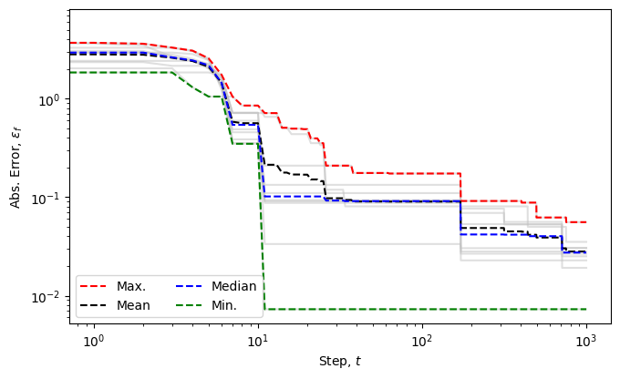
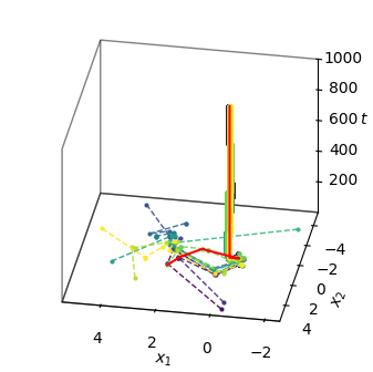
fig = plt.figure(figsize=(width/2, width/2))
ax = fig.add_subplot(111, projection='3d')
ax.set_proj_type('ortho')

cmap = plt.get_cmap('viridis', num_agents)
color = cmap(np.linspace(0, 1, num_agents))

steps = np.arange(optimiser._num_iterations) + 1

for agent, c in enumerate(color):
    ax.plot3D(positions[:, agent, 0], positions[:, agent, 1], steps,
              "--o", color=c, alpha=0.9, markersize=2, linewidth=1,
              label=f"Agent {agent}")

ax.plot3D(best_position[:, 0], best_position[:, 1], steps,
          "-", color="red", markersize=2,  linewidth=1.5,
          label="Best position")

for axis in [ax.xaxis, ax.yaxis, ax.zaxis]:
    axis.pane.set_edgecolor('black')
    axis.pane.set_linewidth(1.0)

# ax.viewfig, _init(elev=35, azim=135)
ax.view_init(elev=30, azim=100)
# ax.legend()
ax.set_xlabel(r"$x_1$", labelpad=1)
ax.set_ylabel(r"$x_2$", labelpad=1)
ax.set_zlabel(r"$t$", labelpad=0)
ax.set_box_aspect([1, 1, 0.8])

ax.set_zlim(1, num_steps)

ax.grid(False)
ax.xaxis.pane.fill = False
ax.yaxis.pane.fill = False
ax.zaxis.pane.fill = False

ax.patch.set_alpha(0)
fig.subplots_adjust(left=0.1, right=0.95, top=0.95, bottom=0.1)

ax.patch.set_alpha(0)
fig.tight_layout()
plt.show()
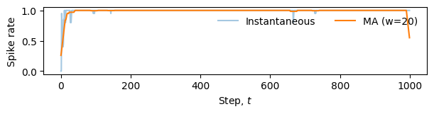
# Spike rate analysis
window = max(5, num_steps // 50)  # choose a small window
# mean activity per step (across agents and dims)
rate = spikes.mean(axis=(1, 2)).astype(float)

# simple moving average
kernel = np.ones(window) / window
rate_ma = np.convolve(rate, kernel, mode='same')

fig, ax = plt.subplots(figsize=(width*0.9, height*0.4))
ax.plot(np.arange(num_steps), rate, alpha=0.4, label="Instantaneous")
ax.plot(np.arange(num_steps), rate_ma, linewidth=1.5, label=f"MA (w={window})")

ax.set_xlabel(r"Step, $t$")
ax.set_ylabel(r"Spike rate")
ax.legend(loc="upper right", ncol=2, frameon=False)

ax.patch.set_alpha(0)
fig.tight_layout()
plt.show()